MSIS 110: Introduction
to Computers
Homework 2: Excel -Creating a Current and Projected
Quarterly Analysis Worksheet
(Excel Project 1 -3 were handed out earlier)
Due date: 06/16/03
|
1.
Read all instructions. 2.
Please follow all the instruction provided
in this handout and in previous handouts.
3.
You will lose some or all credit if your
answer is correct, but you did not follow the instructions.
|
Purpose: To demonstrate the ability to create a data series, use the Format Painter button, copy a range
to a nonadjacent range, apply formulas that use absolute referencing, create a
chart, use goal seeking, and perform what-if analysis.
Problem: You are the accountant for
JJW Discount Warehouse. The president of the company, JW, is concerned that the
store is carrying too many customers on its own in-store credit accounts
(referred to as FE Accounts). He has asked you to create a worksheet for the
second quarter of sales that depicts the amount of sales by cash, bank cards
(referred to as BC), credit through a local finance company (referred to as
Finance Co.), and layaway. Furthermore, he wants to see projected third quarter
sales. Finally, the worksheet should show the percent of total sales by each
type of payment for April, May, and June.
Part 1 Instructions: Perform the following
tasks to create the worksheet in Figure E3A-1.
1. Bold the entire worksheet. Enter the worksheet title, JJW
Discount Warehouse, in cell A1. Enter a subtitle, Quarterly Sales Analysis, in
cell A2. Change the height of rows 1 and 2 to 18.00 points.
2. Change the font of cells A1 and A2 to any available font besides
Arial or Times New Roman.
3. Center the two titles across columns A through G.
4.
Change the background color of the first two rows to aqua
(column 5, row 3 of the Color palette) and the color of the text to white.
5. Enter the words, Prepared by, followed by your full name in cell
A3 and your Student ID or SSN. Enter the
NOW function in cell G3, and change the format to dd-mmm-yy
style.
6. Enter the words, Second Quarter Sales, in cell A4 and the words,
Projected Third Quarter Sales, in cell E4.
7. Enter the first month of the third quarter,
APR, in cell B5 and right-align it. Use the fill handle to create the month
series in row 5, so the headings read APR through SEP.
8. Change the column headings’ background colors in row 5 to sky
blue (column 6, row 4 of the Color palette).
9. Enter the row titles from Table E3A-1 below, starting in cell A6.
10. Change the width of column A to 12.00 points and of columns B
through G to 10.57 points.
11.
Use the data in Table E3A-1
below in the range B6:D10 as a basis for creating your own data set.
ü
Assume that your Student
ID/SSN is 999-99-0123.
ü
The last three digits are
123.
ü
Use this value to adjust
all the values provided in table E3A-1.
ü
Failure to do so will
result in zero points for the entire assignment. The values that you use must be from your own
Student ID/SSN.
ü
Your cash in April will be: 11,985.00 + 123.00 = 12,108.00
ü
Make sure that you enter
the equation in the appropriate cell (such as B6 for April Cash)
For B6=> =
11,985.00 + 123.00 and NOT 12,108.00
ü
Your FE accounts in June
will be: 7,613.36 + 123.00 = 7,736.36
Format
the range B6:G10 to Comma style with two decimal places.
|
|
APR |
MAY |
JUN |
|
Cash |
11,985.00 |
10,697.00 |
11,357.00 |
|
BC |
9,951.19 |
10,624.16 |
9,852.19 |
|
FE Accts |
7,384.36 |
8,212.04 |
7,613.36 |
|
Finance
Co. |
4,582.57 |
4,127.48 |
4,546.57 |
|
Layaway |
609.74 |
681.36 |
673.74 |
Table E3A-1
12. The projected third quarter sales are based on previous quarter’s
sales. To calculate the month of July, increase June sales by 1.5 percent.
August is expected to have a 3.0 percent increase over July sales, and
September is expected to have a 5.5 percent increase over August. Enter the appropriate following formulas
in the designated cells: E6, F6, and G6. Use the fill handle to copy
the formulas for each column.
13. Enter the title, Total Sales, in cell A11 and
change the background colors in the range A11:G11 to yellow. Use the SUM
function to calculate the total sales for April. Use the fill handle to copy
the sum for all the columns. Format the range B11:G11 to comma style with two
decimal positions.
14. Complete the following entries.
a.
In cell A12, enter the title, Analysis
b.
Copy the labels for the five types of sales, Cash, BC, FE Accts, Finance
Co., and Layaway, from cells A6:A10 to A13:A17
c.
Calculate the percentages for each of the five types of sales by
dividing the APR value by the Total. use an appropriate equation.
d. Use the fill handle to copy the
formula down to cell B17. Format these cells as Percent with no decimal places
e. Create similar entries for MAY and JUN in
columns C and D
f.
Change the color of the range A12:D17 to gray-25%
g. Adjust the height of row 12 to
21.00 point
15. Enter your name in cell A20. In the cells
directly below your name, enter your course identification, computer lab
assignment (Excel Homework), date, and instructor name.
16. Rename the Sheet 1 tab, Analysis.
17. Save the workbook using the file name, Yourname - ExcelHomework –Part1,
where Yourname is your own last name. I will save my work as:
e.g.: Mathiyalakan-ExcelHomework-Part1
18. Preview and print the worksheet. Preview and
print the formulas (CTRL+`) in landscape orientation using the Fit to option
button in the Page Setup dialog box.
19. Redisplay the values version of the
worksheet.
Part 2 Instructions: Using Chart Wizard, draw the 3D column chart illustrated in
Figure E3A-2 showing the monthly amount of sales based on JJW Discount
Warehouse’s customer credit (FE Accts). This chart uses the nonadjacent ranges
B5:G5 (category) and B8:G8 (data series). Place this chart on a separate sheet.
Make the following modifications to the chart.
1. Double underline the chart title and make its font size 24 point.
2. Adjust the Y-axis labels to a font size of 12 point.
3. Change the color of the columns to green.
4. Rename the tab for the chart to Credit Chart. Rearrange the tabs
so Analysis is before Credit Chart.
5. Delete unused sheets and save the workbook again.
6. Print both sheets.
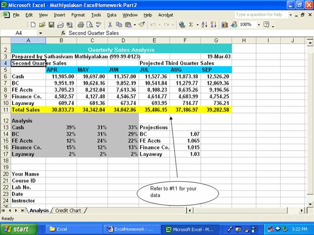
Part 3 Instructions:
1. You determine that the increases for each type of sale may not be
the same. You need to add an additional area to the worksheet called
Projections. Enter the label, Projections, in cell E13. Put the data from Table
E3A-2 in cells E14:F17.
|
Projections |
|
|
BC |
1.07 |
|
FE Accts |
1.065 |
|
Finance
Co. |
1.015 |
|
Layaway |
1.03 |
Table E3A - 2
2. Modify the formulas used for noncash
third quarter projections in cells E7:G10. Using absolute references, update
the July formulas using the projections in the range F14:F17. Use the fill
handle to copy these formulas across for August and September sales.
3. JW is concerned that too many sales are made on in-house charge
accounts. Use the Goal Seek command to determine the FE Accts amount for April,
if the percentage is to be only 12%.
4. Save the workbook as Yourname
- ExcelHomework -Part2, where Yourname
is your own last name. I will save my
work as:
e.g.:
Mathiyalakan-ExcelHomework-Part2
5. Print this revised Analysis sheet. It should display as shown in
Figure E3A-3.
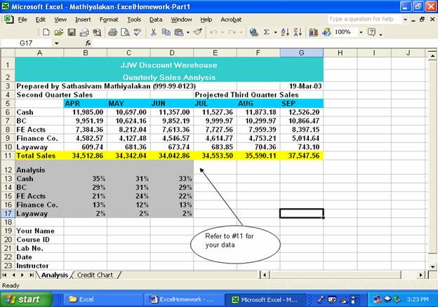
Figure E3A - 1
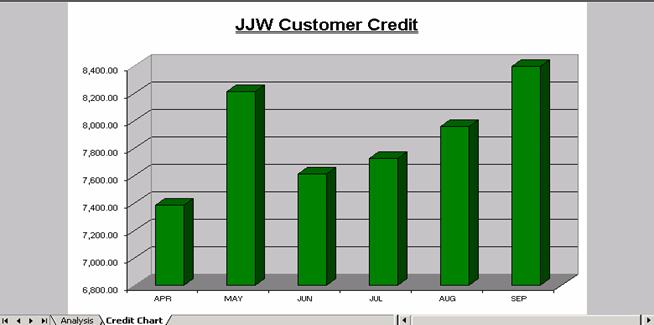
Figure E3A - 2